Note that we will follow a very similar structure as we have done in the chapter for discrete variable. And, indeed, a lot of the theorems can be directly transported to the continuous case. However, analysis of the continuous variables are slightly harder since, as one might expect, all the summation no becomes integral.
This chapter will first goes from the definition of continuous random variable with link established via the cumulative distribution functions. Then, we will go over some of the common continuous distributions.
2 Cumulative Distribution
Definition 1 The (cumulative) distribution function (cdf) of a random variable \(Y\) is \[
F(y) = P(Y \leq y)
\]
Theorem 1 if \(F(y)\) is a cdf then: 1. \(F(y) \to 0\) as \(y \to - \infty\) 2. \(F(y) \to 1\) as \(y \to \infty\) 3. \(F(y)\) is nondecreasing.
Note that we assumes that \(F(y)\) is right continuous, meaning that \(\lim_{\delta \to 0} F(Y + \delta) = F(y)\).
3 Random Variable
Armed with cdf, we are now ready to define what continuous random variable is.
Definition 2 A random variable is said to be continuous if its cdf is continuous (everywhere).
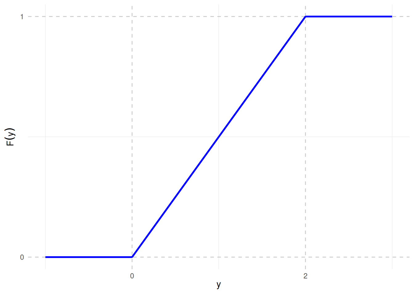
Example 1 Let \(Y\) be a number chosen randomly between 0 and 2. Find \(Y\)’s cdf. Is \(Y\) a continuous random variable.
\[
F(y) = \begin{cases}
0 & y < 0 \\
y/2 & 0 \leq y < 2 \\
1 & y \geq 2
\end{cases}
\]
Show the code
library(ggplot2)y <-seq(-1, 3, length.out =400)F <-ifelse(y <0, 0, ifelse(y <2, y/2, 1))df <-data.frame(y = y, F = F)ggplot(df, aes(x = y, y = F)) +geom_line(color ="blue", linewidth =1) +labs(x =expression(y), y =expression(F(y))) +scale_x_continuous(breaks =c(0, 2)) +scale_y_continuous(breaks =c(0, 1)) +theme_minimal() +theme(panel.grid.major =element_line(linetype ="dashed", color ="grey80"))
Observe that \(F(y)\) is continuous everywhere (i.e. for all \(y\) between \(-\infty\) and \(\infty\)). Hence \(Y\) is a continuous random variable.
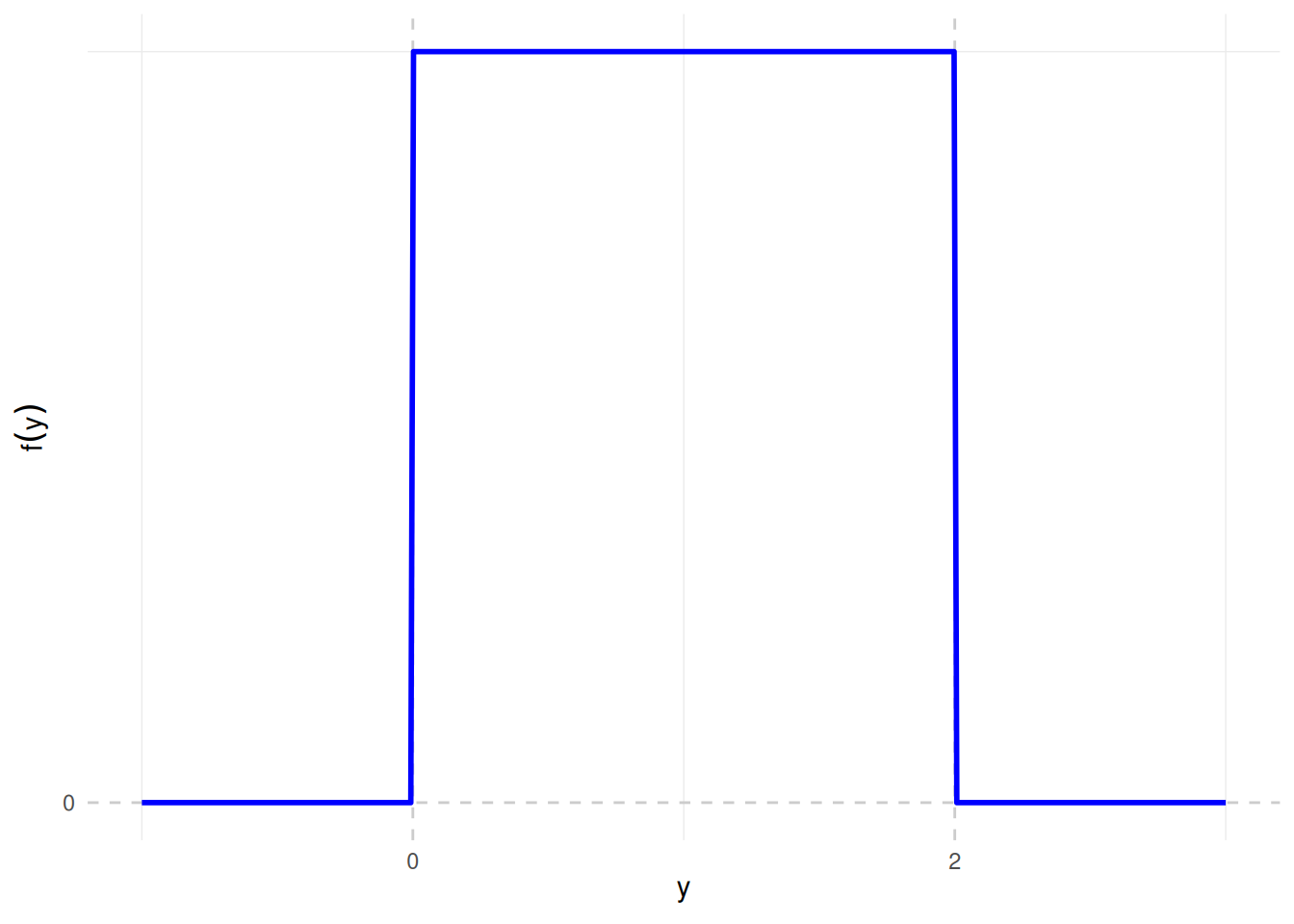
4 Probability Density Function
Note that if \(Y\) is continuous, then \(P(Y = y) = 0 \; \forall y\). Therefore, we need to redefine something instead of the previously defined pmf as it is now useless.
Definition 3 Suppose that \(Y\) is continuous random variable with cdf \(F(y)\). Then \(Y\)’s probability density function is \[
f(y) = F'(y) = \frac{dF(y)}{dy}
\]