Interval Estimation

Published

Sunday Jun 8, 2025

1 Motivation

There are times when a point estimate is not really helpful simply because it only provides one number. It does not provide any form of statistical confidence to how good the inference is. How wrong might it be if it were to deviate? Also, loosely speaking, the probability that we make a correct guess for the parameters, which would typically be continuous, is $0$. Therefore, we may want an interval on the axis instead.

2 Interval Estimation and Confidence Intervals

Consider a sample $Y_1, Y_2, \ldots, Y_n$ from a probability distribution which depends on one parameter $\theta$ (which is fixed but unknown).

Now, we want to find two function $g$ and $h$ such that \[\begin{gather} L = g(Y_1, Y_2, \ldots , Y_n) \nonumber \\ U = h(Y_1, Y_2, \ldots , Y_n) \\ \end{gather}\] would satisfy the following probability statement¹ \[\begin{equation} P(L \leq \theta \leq U) = 1 - \alpha \end{equation}\] Then, $[L, U]$ is a $100(1 - \alpha)%$ confidence interval (CI) for $\theta$ in which $L$ and $U$ are the lower and upper bound and $1 - \alpha$ is the coverage coefficient, of the CI.

Example 1 (Confidence Interval for Continuous Uniform) Suppose that 6.2 is a number chosen randomly between $0$ and $c$. Find an $80\%$ confidence interval for $c$.

Solution:

Let $Y \sim U(0, c)$. Then, $X = Y/c \sim U(0, 1)$ by applying the transformation method.

Definition 1 (Pivotal Quantity) Then, we call $X$ a pivotal quantity. This means that $X$ is a function of $Y$ the observable random variables and $c$, the estimand, whose distribution does not depend on $c$.

This quantity is useful for finding the confidence interval.

Therefore, for an $80\%$ confidence interval for $c$, \[\begin{align*} 0.8 = \P{0.1 \leq X \leq 0.9} & = \P{0.1 \leq Y / c \leq 0.9} \\ & = \P{10Y/9 \leq c \leq 10Y} \end{align*}\]

So $[10Y/9, 10Y]$ is an $80\%$ CI for $c$.

Now, since the realised value of $Y$ is $y = 6.2$, we have an interval estimation being $[6.82, 62]$.

Note that the term ‘confidence interval’ refers to both $[10Y/9 , 10Y]$ and $[10y / 9, 10y]$; the former is a random variable and the latter is the realised value of that random variable.

We should also note that whether to include the endpoint, even though does not matter for the current case as $X$ is continuous, it can be important in some cases.

Note 1: A smart Alternative to Example 1

Solution. First, notice that in order to obtain the center $80\%$ of $U(0, c)$, we need the center $80\%$ of the sample space of the distribution, which is $[0, c]$. Therefore, with some attention, such interval in the probability statement would then be \[\begin{equation*} \P{0.1c \leq Y \leq 0.9c} = 0.8 \end{equation*}\] Then, the following follows.

2.1 Interpretation of CI

Can we really say that $c$ lies between $6.89$ and $62$ with probability $80\%$?

No. The event “6.89 < c < 62” does not involve any random variables. It is either true or false, and so its probability must be either $1$ or $0$, respectively, and not $0.8$. Thus the statement $\P{6.89 < c < 62} = 0.8$ is wrong.

The way to interpret ‘$80\%$ confident’ is as follows. If we were to sample another number, e.g. $5.4$ from the same $U(0, c)$ distribution, then we’d get another CI, e.g. $(10(5.4)/9, 10(5.4)) = (6, 54)$. Now imagine sampling very many such numbers, so as to get the same number of corresponding CIs, e.g. $(6.89, 62)$, $(6, 54)$, $(8.89, 80)$, $\ldots$. Then close to $80\%$ of these CIs will contain $c$. This is an expression of the fact that $\P{10Y/9 < c < 10Y} = 0.8$. But for any particular value $y$ of $Y$, we should never write $\P{10y/9 < 10y} = 0.8$.

2.2 Upper and Lower Range CIs

The $80\%$ CI derived above, $(10Y/9, 10Y)$, may also be called a central CI. It is also possible to construct other types of CI. Three major types are defined as follows

Let $I = [L, U] = [g(Y_1, Y_2, \ldots , Y_n), h(Y_1, Y_2, \ldots , Y_n)]$ be a $100(1 - \alpha)\%$ confidence interval for $\theta$. Thus $P(L \leq \theta \leq U) = 1 - \alpha$ for all $\theta$.

2.2.1 Upper Range Confidence Interval

We say that $I$ is an upper range confidence interval if \[\begin{equation} \P{\theta \geq L} = 1 - \alpha \hspace{10pt} (= \P{L \leq \theta} = \P{L \leq \theta \leq \infty}) \end{equation}\]

Then $\P{\theta < L} = \alpha$, $U = \infty$ and we call $L$ the $1 - \alpha$ lower confidence limit for $\theta$.

2.2.2 Lower Range Confidence Interval

We say that $I$ is a lower range confidence interval if \[\begin{equation} \P{\theta \leq L} = 1 - \alpha \hspace{10pt} (= \P{L \geq \theta} = \P{- \infty \leq \theta \leq U}) \end{equation}\]

Then $\P{\theta > U} = \alpha$, $L = -\infty$ and we call $U$ the $1 - \alpha$ upper confidence limit for $\theta$.

2.2.3 Central Confidence Interval

We say that $I$ is a central confidence interval if \[\begin{equation} \P{\theta < L} = \P{\theta > U} = \alpha / 2 \end{equation}\]

Example 2 Check that $[10Y/9, 10Y]$ is central $80\%$ CI for $c$.

Solution. \[\begin{gather*} \P{\theta < L} = \P{c < 10Y/9} = \P{Y > 0.9c} = 0.1 = \alpha / 2 \\ \P{\theta > U} = \P{c > 10Y} = \P{Y < 0.1c} = 0.1 = \alpha / 2 \\ \end{gather*}\]

Example 3 (Example 5) Now, we know that Example 2 is the central confidence interval. Therefore, if we can also ask the question about lower and upper confidence interval.

Solution. \[\begin{equation*} 0.8 = \P{X \leq 0.8} = \P{Y/c \leq 0.8} = \P{5Y / 4 \leq c} \end{equation*}\]

So $L = 5Y / 4$, with realised value $5(6.2) / 4 = 7.75$. So an upper range $80\%$ CI for $c$ is $[7.75, \infty)$.

What is a lower range $80\%$ CI for $c$?

\[\begin{equation*} 0.8 = \P{X \geq 0.2} = \P{Y/c \geq 0.2} = \P{c \leq 5Y} \end{equation*}\]

So $U = 5Y$, with realised value $5(6.2) = 31$. So a lower range $80\%$ CI for $c$ is $(-\infty, 31]$.

However, we can actually refine the lower and upper confidence interval…

First, observe that $c$ cannot be negative. So a lower range $80\%$ CI for $c$ is $[0, 31]$. Secondly, we also know that $0 \leq y \leq c$, and therefore $c \geq y = 6.2$. So a lower range $80\%$ CI for $c$ is $[6.2, 31]$.

Lower range $80\%$ CI $= [6.2, 31]$
Upper range $80\%$ CI $= [7.75, \infty)$
Central $80\%$ CI $= [6.89, 62]$

Note that the lower range CI is the shortest of the three. This is an attractive property, and sometimes we may choose one CI formula over another because it leads to a shorter CI on average. However, in some cases (not considered here), choosing the shortest of two or more CIs only after observing the data (as is sometimes done) may cause the confidence conefficient to be altered so that it is no longer the nominal $1-\alpha$.

Example 4

Example 4 Suppose that $1.2$, $3.9$ and $2.4$ are a random sample from a normal distribution with variance $7$. Find a $95\%$ confidence interval for the normal mean.

Solution. We cannot rely on the intelligence of finding a smart alternative as Note 1.

Let $Y_1, Y_2, \ldots , Y_n \sim^\iid \NormalDist(\mu, \sigma^2)$. Let’s find a $100(1 - \alpha)\%$ CI for $\mu$ generally. Recall that $Z = \frac{\mean{Y} - \mu}{\sigma / \sqrt{n}} \sim \NormalDist(0, 1)$. Therefore, $Z$ is a pivotal quantity, \[\begin{align*} 1 - \alpha & = \P{-z_{\alpha/2} < Z < z_{\alpha/2}} \\ & = \P{-z_{\alpha/2} < \frac{\mean{Y} - \mu}{\sigma / \sqrt{n}} < z_{\alpha/2}} \\ & = \P{-z_{\alpha/2}\frac{\sigma}{\sqrt{n}} < \mean{Y} - \mu < z_{\alpha/2}\frac{\sigma}{\sqrt{n}}} \\ & = \P{\mean{Y}-z_{\alpha/2}\frac{\sigma}{\sqrt{n}} < \mu < \mean{Y} + z_{\alpha/2}\frac{\sigma}{\sqrt{n}}} \\ \end{align*}\]

So a $100(1 - \alpha)\%$ CI for $\mu$ is $(\mean{Y} - z_{\alpha/2}\frac{\sigma}{\sqrt{n}} , \mean{Y} + z_{\alpha/2}\frac{\sigma}{\sqrt{n}})$. This interval may also be written $\mean{Y} \pm z_{\alpha/2}\frac{\sigma}{\sqrt{n}}$.

In our case: $100(1 - \alpha) = 95 \to \alpha = 0.05$. Therefore $z_{\alpha/2} = z_{0.025} = 1.96$
$n = 3$
$\mean{y} = \frac{1}{n} \sum_{i=1}^n y_i = \frac{1}{3}(1.2 + 3.9 + 2.4) = 2.5$
$\sigma^2 = 7$

So the $95\%$ CI for $\mu$ is \[\begin{equation*} (\mean{y} \pm z_{\alpha / 2}\frac{\sigma}{\sqrt{n}}) = \left(2.5 \pm 1.96 \frac{\sqrt{7}}{\sqrt{3}}\right) = (2.5 \pm 3.0) = (-0.5, 5.5) \end{equation*}\]

Example 7

Example 5 Suppose the same sample with Example 4 but unknown variance. Find a $95\%$ confidence interval for the normal mean.

Solution. Let $Y_1, Y_2, \ldots ,Y_n \sim^\iid \NormalDist(\mu , \sigma^2)$. Recall that \[\begin{equation} T = \frac{\mean{Y} - \mu}{S / \sqrt{n}} \sim t(n-1) \end{equation}\] with $T$ being the pivotal quantity.

Therefore, \[\begin{align*} 1 - \alpha & = \P{-t < T < t} \tag{where $t = t_{\alpha/2}(n - 1)$} \\ &= \P{ -t < \frac{\mean{Y} - \mu}{S / \sqrt{n}} < t } \\ &= \P{ \mean{Y} - t\frac{S}{\sqrt{n}} < \mu < \mean{Y} + t\frac{S}{\sqrt{n}} } \\ \end{align*}\]

So a $100(1-\alpha)\%$ CI for $\mu$ is $\left( \mean{Y} \pm t_{\alpha/2}\!(n-1) \frac{S}{\sqrt{n}} \right)$

With some algebraic calculation we have, the $95\%$ CI is \[\begin{gather*} 100(1 - \alpha) = 95 \implies \alpha = 0.05, \, n = 3 \\ t_{\alpha / 2}(n - 1) = t_{0.025}(2) = 4.303 \\ \mean{y} = \frac{1}{n} \sum_{i=1}^n y_i = \frac{1}{3} (1.2 + 3.9 + 2.4) = 2.5 \\ s^2 = \frac{1}{n-1} \left( \sum_i y_i^2 - 3 * (\mean{y})^2 \right) = 1.83 \\ \end{gather*}\] So the $95\%$ CI for $\mu$ is $(-0.86k 5.86)$.

Note that the interval for Example 5 is wider than the CI in Example 3, $(-0.5, 5.5)$. This corresponds to the fact that $\sigma$ is now unknown and effectively needs to be estimated from the sample, by $s$. This illustrates the fact that when information is decreased, CI’s tend to become wider (which makes sense because there is greater uncertainty). However, this is not always the case, and sometimes a decrease in information can, by change, lead to an interval (with the same confidence coefficient) which much narrower.

Approximation with Sample Variance

Example 6 200 people were randomly sampled from the population of Australia, and their heights were measured. The sample mean was 1.673 and the sample standard deviation was 0.310.

Find a $95\%$ confidence interval for the average height of all Australian.

First, in summary of the above, we know,

$Y_i \iid (\mu, \sigma^2)$ where $\mu$ and $\sigma$ unknown
$\mean{Y} = 1.673$
$S = 0.310$

Solution. Let $Y_i$ be the $i$th height and assume that $Y_1, Y_2, \ldots , Y_n \sim^\iid (\mu, \sigma^2)$. Now, by central limit theorem, $\frac{\mean{Y} - \mu}{\sigma / \sqrt{n}} \approx \NormalDist(0, 1)$ as $n = 200$ is large. But $\sigma$ is unknown, and so we cannot make use of this pivotal quantity.

However, recall that the $t = \frac{\mean{Y} - \mu}{S / \sqrt{n} \sim t(n-1) \dconv \NormalDist(0, 1)}$. This idea will be more thoroughly explore in Chapter 9. For now, we can approximate with \[\begin{equation*} Z = \frac{\mean{Y} - \mu}{S / \sqrt{n}} \approx \NormalDist(0, 1) \end{equation*}\] also. Using the same logic as in the last few examples, we find that $100(1 - \alpha)\%$ CI for $\mu$ is $\left(\mean{Y} \pm z_{\alpha / 2} \frac{S}{\sqrt{n}}\right)$, which in our case is $(1.630, 1.716)$.

Note that this is only an approximate CI. However, the closeness of the approximation will be very good if $n$ is large. Also, we would definitely replace $S$ with $\sigma$ if the population standard deviation is known.

3 Discrete Cases

Motivating Example towards Wilson CI

Example 7 Suppose that we toss a bent coin 100 times and get 72 heads. Find the 95% confidence interval for the probability of a head.

Solution. Let $Y =$ number of heads out of the $n = 100$ tosses and $p =$ probability of a head on a single toss.

Then $Y \sim \Binomial(n, p)$, with realised value $y = 72$. Now $Y \approx \NormalDist(np, np(1 - p))$ as a result of central limit theorem as $n = 100$ is large. Therefore, applying standardisation, \[\begin{equation*} \frac{Y - np}{\sqrt{np(1-p)}} \approx \NormalDist(0, 1) \end{equation*}\]

\[\begin{align*} 1 - \alpha &\approx \P{-z_{\alpha / 2} < \frac{Y - np}{\sqrt{np(1 - p)}} < z_{\alpha/2}} \\ &\approx \P{-z_{\alpha / 2} < \frac{Y - np}{\sqrt{n\hat{p}(1 - \hat{p})}} < z_{\alpha/2}} \\ &\approx \P{\frac{Y}{n} - z_{\alpha / 2} \sqrt{\frac{\hat{p}(1 - \hat{p})}{n}} < p < \frac{Y}{n} + z_{\alpha / 2} \sqrt{\frac{\hat{p}(1 - \hat{p})}{n}}} \\ \end{align*}\]

So a $100(1 - \alpha)\%$ CI for $p$ is $\left( \hat{p} \pm z_{\alpha / 2}\sqrt{\frac{\hat{p}(1 - \hat{p})}{n}} \right)$.

IN our case $\hat{p} = y/n = 72/100 = 0.72$, and so the required $95\%$ CI is $\left( 0.72 \pm 1.96\sqrt{\frac{0.72(1-0.72)}{100}} \right) = (0.72 \pm 0.09) = (0.63, 0.81)$.

Since this interval is entirely above $0.5$, we can reasonably suspect that the coin is not fair and that heads are more likely to come up than tails.

The CI above is called the standard CI for a binomial proportion. It is only one amongst many that have been proposed in the statistical literature. The following is another one which is more complicated but arguably better.

3.1 Wilson CI for a Binomial Proportion

Now, in fact the following is another way of estimation the interval.

Theorem 1 (Wilson CI) Another $100(1-\alpha)\%$ CI for $p$ is given by \[\begin{equation} \left( \frac{\hat{p} + \frac{z^2_{\alpha/2}}{2n} \pm z_{\alpha / 2} \sqrt{\frac{\hat{p}(1-\hat{p})}{n} + \frac{z^2_{\alpha/2}}{4n^2}}}{1 + \frac{z^2_{\alpha/2}}{n}} \right) \end{equation}\]

This interval is called the Wilson CI for a binomial proportion. Note that if $n$ is large this CI is approximately the same as the standard CI introduced in Example 7.

Proof. Observe that \[\begin{align*} 1 - \alpha &\approx \P{-z_{\alpha / 2} < \frac{Y - np}{\sqrt{np(1 - p)}} < z_{\alpha/2}} \\ &= \P{\left(\frac{Y - np}{\sqrt{np(1 - p)}}\right)^2 < z^2} \tag{where $z = z_{\alpha/2}$} \\ &= \P{ Y^2 - 2npY + n^2 p^2 < z^2 np - z^2 np^2 } \\ &= \P{ p^2\left(1 + \frac{z^2}{n}\right) - p\left(\frac{2Y}{n} + \frac{z^2}{n} \right) + \frac{Y^2}{n^2} < 0 } \\ &= \P{ p^2\left(1 + \frac{z^2}{n}\right) - p\left(2\hat{p} + \frac{z^2}{n} \right) + \hat{p}^2 < 0 } \tag{where $\hat{p} = \frac{Y}{n}$} \\ &= \P{ a < p < b }, \\ \end{align*}\] where $a$ and $b$ are the roots of quadratic function $\eqref{eq:root-quad-func}$. \[\begin{equation} \label{eq:root-quad-func} f(p) = p^2\left( 1 + \frac{z^2}{n} \right) - p\left(2\hat{p} + \frac{z^2}{n}\right) + \hat{p}^2 \end{equation}\] Hence, finding the roots of $\eqref{eq:root-quad-func}$ yield, \[\begin{align*} & \frac{ (2\hat{p} + \frac{z^2}{n}) \pm \sqrt{(2\hat{p} + \frac{z^2}{n})^2 - 4\hat{p}^2(1 + \frac{z^2}{n})} }{ 2(1 + \frac{z^2}{n}) } \\ &= \frac{ \hat{p} + \frac{z^2}{2n} \pm \frac{1}{2} \sqrt{ 4\hat{p}^2 + \frac{4\hat{p} z^2}{n} + \frac{z^4}{n^2} - 4\hat{p}^2 - \frac{4\hat{p}^2 z^2}{n} } }{ 1 + \frac{z^2}{n} } \\ &= \frac{ \hat{p} + \frac{z^2}{2n} \pm \sqrt{ \frac{\hat{p} z^2}{n} + \frac{z^4}{4n^2} - \frac{\hat{p}^2 z^2}{n} } }{ 1 + \frac{z^2}{n} }\\ \end{align*}\]

Example 9 in Wilson CI

Example 8 Find the Wilson CI for the same setting as Example 7.

Solution. \[\begin{equation} \left( \frac{0.72 + \frac{1.959964^2}{2\cdot 100} \pm 1.959964 \sqrt{\frac{0.72(1-0.72)}{100} + \frac{1.959964^2}{4\cdot100^2}}}{1 + \frac{1.959964^2}{100}} \right) = \frac{0.739207 \pm 0.009007}{1.0384} = (0.625, 0.798) \end{equation}\]

Note that the above is very similar to the standard CI $(0.63, 0.81)$ derived in Example 7.

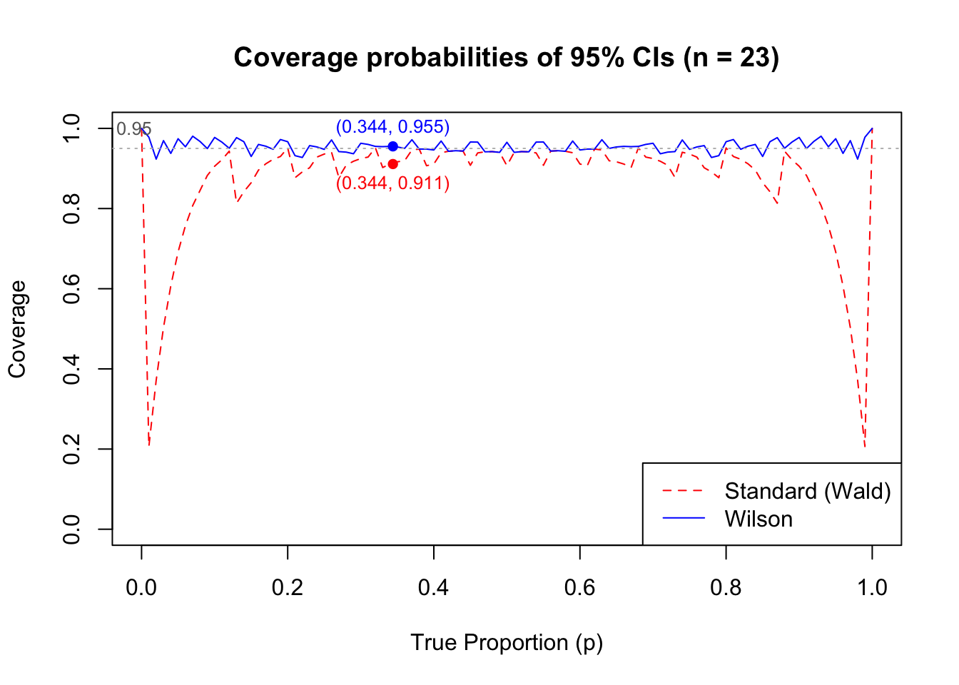
3.2 Why is Wilson CI is better?

The Wilson CI is considered ‘better’ than the standard CI because its coverage probabilities are overall closer to the desired $1 - \alpha$. For example, if $n = 23$ and $p = 0.344$, the coverage probability of the standard $95\%$ CI is $91.4\%$, and the coverage probability of the Wilson $95\%$ CI is $95.5\%$. These calculations can be repeated for all values of $p$ on a grid ($p = 0.001, 0.002, \ldots , 1$), with $n = 23$ held the same in each case.

Essentially, this is because the Wald interval uses $\hat{p}$ to approximate $p$ multiple times to obtain the interval estimation. Particularly, the approximation is used in the “standard error” part for the test statistic. In another perspective, the sample size can be seen as the key factor because it is essentially providing more information to $\hat{p}$ to approximate $p$ with a more accurate approximation.

From Figure 1, it is clear that as $p$ become more “extreme” values, the Wald CI fails quite dramatically. This is because such $p$ values usually result in a asymmetric distribution, particularly with small $n$ like $23$².

Show the code

# Set parameters
n <- 23
alpha <- 0.05
z <- qnorm(1 - alpha/2)
p_vals <- seq(0, 1, by = 0.01)

# Function to compute Wald CI
wald_ci <- function(y, n) {
  phat <- y / n
  se <- sqrt(phat * (1 - phat) / n)
  lower <- phat - z * se
  upper <- phat + z * se
  c(lower, upper)
}

# Function to compute Wilson CI
wilson_ci <- function(y, n) {
  phat <- y / n
  center <- (phat + z^2 / (2 * n)) / (1 + z^2 / n)
  margin <- z / (1 + z^2 / n) * sqrt(phat * (1 - phat) / n + z^2 / (4 * n^2))
  lower <- center - margin
  upper <- center + margin
  c(lower, upper)
}

# Compute coverage for each p
wald_coverage <- numeric(length(p_vals))
wilson_coverage <- numeric(length(p_vals))

for (i in seq_along(p_vals)) {
  p <- p_vals[i]
  probs <- dbinom(0:n, n, p)
  
  wald_hits <- 0
  wilson_hits <- 0
  
  for (y in 0:n) {
    wald_bounds <- wald_ci(y, n)
    wilson_bounds <- wilson_ci(y, n)
    
    # Count if p is inside the interval
    if (p >= wald_bounds[1] && p <= wald_bounds[2]) {
      wald_hits <- wald_hits + probs[y + 1]
    }
    if (p >= wilson_bounds[1] && p <= wilson_bounds[2]) {
      wilson_hits <- wilson_hits + probs[y + 1]
    }
  }
  
  wald_coverage[i] <- wald_hits
  wilson_coverage[i] <- wilson_hits
}

# Plot
plot(p_vals, wald_coverage, type = "l", col = "red", lty = 2, ylim = c(0, 1),
     xlab = "True Proportion (p)", ylab = "Coverage",
     main = "Coverage probabilities of 95% CIs (n = 23)")
lines(p_vals, wilson_coverage, col = "blue", lty = 1)
abline(h = 0.95, col = "gray", lty = 3)
text(-0.01, 0.95, labels = "0.95", pos = 3, col = "gray40", cex = 0.8)

legend("bottomright", legend = c("Standard (Wald)", "Wilson"),
       col = c("red", "blue"), lty = c(2, 1))

# Highlight example point
p_example <- 0.344
ix <- which.min(abs(p_vals - p_example))
points(p_example, wald_coverage[ix], col = "red", pch = 16)
points(p_example, wilson_coverage[ix], col = "blue", pch = 16)
text(p_example, wald_coverage[ix], 
     labels = paste0("(", p_example, ", ", round(wald_coverage[ix], 3), ")"),
     pos = 1, col = "red", cex = 0.8)
text(p_example, wilson_coverage[ix], 
     labels = paste0("(", p_example, ", ", round(wilson_coverage[ix], 3), ")"),
     pos = 3, col = "blue", cex = 0.8)

4 Difference of $p$ in Binomial

Theorem 2 (Difference in Proportion) Let $X \sim \Binomial(n, p)$, and $Y \sim \Binomial(m, q)$, where both $n$ and $m$ are large and $X \perp Y$.

Then the approximate (Use of CLT and point estimator) $100(1 - \alpha)\%$ CI for $p - q$ is \[\begin{equation} \left( \hat{p} - \hat{q} \pm z_{\alpha / 2} \sqrt{\frac{\hat{p}(1 - \hat{p})}{n} + \frac{\hat{q}(1 - \hat{q})}{m}} \right) \end{equation}\]

Proof. From CLT, we have:

$\hat{p} \approx \NormalDist\left(p, \dfrac{p(1 - p)}{n} \right)$
$\hat{q} \approx \NormalDist\left(q, \dfrac{q(1 - q)}{m} \right)$

when $n$ and $m$ are large.

So:

\[ \hat{p} - \hat{q} \approx \NormalDist\left(p - q,\ \dfrac{p(1 - p)}{n} + \dfrac{q(1 - q)}{m} \right) \]

Since the sum (or difference) of two normal random variables is also normal, and $\hat{p}$ and $\hat{q}$ are independent, this implies:

\[ \text{Var}(\hat{p} - \hat{q}) = \text{Var}(\hat{p}) + \text{Var}(\hat{q}) \]

Thus:

\[ \frac{\hat{p} - \hat{q} - (p - q)}{ \sqrt{ \dfrac{p(1 - p)}{n} + \dfrac{q(1 - q)}{m} } } \approx \NormalDist(0, 1) \]

and, by substitution of sample estimates for large $n$ and $m$:

\[ \frac{\hat{p} - \hat{q} - (p - q)}{ \sqrt{ \dfrac{\hat{p}(1 - \hat{p})}{n} + \dfrac{\hat{q}(1 - \hat{q})}{m} } } \approx \NormalDist(0, 1) \quad \text{if } n \text{ and } m \text{ are large} \]

Remark 1. Note that this one uses both the CLT and the point estimator to approximate the final solution. Note that for large enough $m$ and $n$, this approximation should converge to something good that is gauranteed by the convergence property that will be discuss in Chapter 9.

Example 10

You have a bent $1 coin and a bent $2 coin.
You toss the $1 coin 200 times and get 108 heads.
You toss the $2 coin 300 times and get 141 heads.

Find a 90% CI for the difference between the probability of a head on the $1 coin and the probability of a head on the $2 coin.

Solution. In our case:

$p$ = probability of heads on a toss of the $1 coin
$q$ = probability of heads on a toss of the $2 coin

\[ \begin{aligned} n &= 200, \quad x = 108, \quad \hat{p} = \frac{108}{200} = 0.54 \\ m &= 300, \quad y = 141, \quad \hat{q} = \frac{141}{300} = 0.47 \\ \alpha &= 0.1, \quad z_{\alpha/2} = z_{0.05} = 1.645 \end{aligned} \]

So a 90% confidence interval for $p - q$ is:

\[ \left( 0.54 - 0.47 \pm 1.645 \sqrt{ \frac{0.54(1 - 0.54)}{200} + \frac{0.47(1 - 0.47)}{300} } \right) \]

\[ = (0.07 \pm 0.075) = (-0.005,\ 0.145) \]

Since this CI contains 0, we suspect the chance of heads is the same for both coins, i.e., the difference is not significantly different from zero. Evidence to support true means are the same/similar to the hypothesis test $p = q$ (i.e. $p - q = 0$).

5 Confidence for Sample Variance

Example 9 (Finding the Confidence Interval for Sample Variance) Suppose that $Y_1, Y_2, \ldots Y_n \sim^\iid \NormalDist(\mu, \sigma^2)$. Find a $100(1 - \alpha)\%$ CI for $\sigma^2$.

Solution. Recall that $\frac{(n-1)S^2}{\sigma^2} \sim \chi^2(n-1)$. Therefore \[\begin{align*} 1 - \alpha &= P\left( \chi^2_{1 - \alpha/2}(n - 1) < \frac{(n - 1)S^2}{\sigma^2} < \chi^2_{\alpha/2}(n - 1) \right) \\ &= P\left( \frac{(n - 1)S^2}{\chi^2_{\alpha/2}(n - 1)} < \sigma^2 < \frac{(n - 1)S^2}{\chi^2_{1 - \alpha/2}(n - 1)} \right) \end{align*}\]

( $\chi^2_p(m)$ is the upper $p$ quantile of the chi square distribution with $m$ degrees of freedom. )

So a $100(1 - \alpha)\%$ CI for $\sigma^2$ is $\left(\frac{(n - 1)S^2}{\chi^2_{\alpha/2}(n - 1)},\frac{(n - 1)S^2}{\chi^2_{1 - \alpha/2}(n - 1)}\right).$

6 Confidence Intervals for the Difference Between Two Population Means

Let:

$X_1, X_2, \ldots, X_n \sim \text{iid } (\mu_X, \sigma_X^2)$ (first sample)
$Y_1, Y_2, \ldots, Y_m \sim \text{iid } (\mu_Y, \sigma_Y^2)$ (second sample)

Assume:

$(X_1, X_2, \ldots, X_n) \perp (Y_1, Y_2, \ldots, Y_m)$ (the two samples are independent)

Define:

$\bar{X} = \frac{1}{n} \sum_{i=1}^n X_i \quad \text{(1st sample mean)}$
$\bar{Y} = \frac{1}{m} \sum_{i=1}^m Y_i \quad \text{(2nd sample mean)}$
$S_X^2 = \frac{1}{n - 1} \sum_{i=1}^n (X_i - \bar{X})^2 \quad \text{(1st sample variance)}$
$S_Y^2 = \frac{1}{m - 1} \sum_{i=1}^m (Y_i - \bar{Y})^2 \quad \text{(2nd sample variance)}$

We wish to construct a $100(1 - \alpha)\%$ confidence interval for $\mu_X - \mu_Y$.
A suitable CI will depend on:

what assumptions we can make regarding the distributions of the $X_i$ and $Y_i$ values
what knowledge we have regarding the two population variances, $\sigma_X^2$ and $\sigma_Y^2$
whether the two sample sizes $n$ and $m$ are ‘large’ (so that we can apply the CLT)

Some Possible CIs for Difference between two Population Means

Here are five different ways…

If $n$ and $m$ are large, and $\sigma_x^2$ and $\sigma_Y^2$ are known, a suitable approximate CI is

\[\begin{equation} \label{eq:basic-diff-mean-ci} \left( \bar{X} - \bar{Y} \pm z_{\alpha/2} \sqrt{ \frac{\sigma_X^2}{n} + \frac{\sigma_Y^2}{m} }\right) \end{equation}\]

If $n$ and $m$ are large, and $\sigma_x^2$ and $\sigma_Y^2$ are both unknown, a suitable approximate CI is

\[\begin{equation} \left( \bar{X} - \bar{Y} \pm z_{\alpha/2} \sqrt{ \frac{S_X^2}{n} + \frac{S_Y^2}{m} }\right) \end{equation}\]

If $X_i$ and $Y_i$ values are normally distributed and $\sigma_x^2$ and $\sigma_Y^2$ are both known, a suitable exact CI is \[\begin{equation} \left( \bar{X} - \bar{Y} \pm z_{\alpha/2} \sqrt{ \frac{\sigma_X^2}{n} + \frac{\sigma_Y^2}{m} }\right) \end{equation}\]

(Same as $\eqref{eq:basic-diff-mean-ci}$, but this one does not rely on CLT)

If the $X_i$ and $Y_i$ values are normally distributed, $\sigma_X^2$ and $\sigma_Y^2$ are unknown, and $n$ and $m$ are both large, a suitable approximate CI is, \[\begin{equation} \left( \bar{X} - \bar{Y} \pm z_{\alpha/2} \sqrt{ \frac{S_X^2}{n} + \frac{S_Y^2}{m} }\right) \end{equation}\]

(Relies on the fact that $t \dconv \NormalDist$.)

If the $X_i$ and $Y_i$ values are normally distributed, all with common population variance $\sigma^2 = \sigma_X^2 = \sigma_Y^2$ which however is unknown, a suitable exact CI is, \[\begin{equation*} \left( \mean{X} - \mean{Y} \pm t_{\alpha/2}(n + m - 2) S_p \sqrt{\frac{1}{n} + \frac{1}{m}} \right). \end{equation*}\]

where $S_p^2 = \frac{(n-1)S_X^2 + (m - 1)S_Y^2}{n+m-2}$ is the pooled sample variance. In fact, $S_p^2$ is unbiased for $\sigma^2$.

If the $X_i$ and $Y_i$ values are normally distributed, nothing at all is known about $\sigma_X^2$ and $\sigma_Y^2$, and $n$ and m are not both large, then the construction of a suitable CI is beyond the scope of this course. Interested students can find out more by researching the Behrens-Fisher problem, e.g. on Wikipedia (this topic is non-assessable).

Footnotes

Note that this cannot really be a probability statement in general. At least under the frequentist viewpoint, the distribution parameter is a fixed, constant rather than a radom variable. Therefore, we would have to “re-interpret” such formula as the percentage of such intervals that would capture the real coefficients if we take a large numbers of random samples and calculate such interval.↩︎
The details of the coverage tests is included in section about coverage test.↩︎