Evaluation Metrics

Published

Sunday Jun 8, 2025

1 Bias

The question now arises: How good is $\hat{p}$ as an estimator of $p$?

What we need are some criteria for assessing the quality of estimators. The bias of an estimator $\hat{\theta}$ of $\theta$ is \[\begin{equation} \bias{\hat{\theta}} = \E{\hat{\theta}} - \theta \end{equation}\]

If $\bias{\hat{\theta}} = 0$, we say that $\hat{\theta}$ is unbiased for $\theta$.

In Example 1, what is the bias of $\hat{p}$? \[\begin{equation*} \E{\hat{p}} = \E{\frac{Y}{n}} = \frac{1}{n} \E{Y} = \frac{1}{n} np = p \end{equation*}\] Therefore, \[\begin{equation*} \bias{\hat{p}} = \E{\hat{p}} - p = p - p = 0 \end{equation*}\]

Hence, we know that $\hat{p}$ is an accurate estimator. But, is $\hat{p}$ also precise?

… but wait, what does it mean to be precise?

Well, precise means that we don’t want to have a highly variational estimator. In other words, we would like the estimator to have an estimate to be relatively close to the target on every sample as well.

2 Precision

Analogy: Target at a firing range:

Show the code

library(MASS)
library(ggplot2)
library(dplyr)
library(tidyr)

mu_accurate <- c(0, 0)
mu_inaccurate <- c(-3, 3)
sigma_accurate <- matrix(data = c(.5, 0, 0, .5), nrow = 2, ncol = 2)
sigma_inaccurate <- matrix(data = c(5, 0, 0, 5), nrow = 2, ncol = 2)

sample_size <- 30

points1 <- mvrnorm(n = sample_size, mu = mu_accurate, Sigma = sigma_accurate)
points2 <- mvrnorm(n = sample_size, mu = mu_accurate, Sigma = sigma_inaccurate)
points3 <- mvrnorm(n = sample_size, mu = mu_inaccurate, Sigma = sigma_accurate)
points4 <- mvrnorm(n = sample_size, mu = mu_inaccurate, Sigma = sigma_inaccurate)

# Combine into a data frame
df <- rbind(
  data.frame(x = points1[,1], y = points1[,2], group = "Accurate & Precise"),
  data.frame(x = points2[,1], y = points2[,2], group = "Accurate & Imprecise"),
  data.frame(x = points3[,1], y = points3[,2], group = "Inaccurate & Precise"),
  data.frame(x = points4[,1], y = points4[,2], group = "Inaccurate & Imprecise")
)

mv <- 7

# Create one plot per group
p1 <- ggplot(filter(df, group == "Accurate & Precise"), aes(x = x, y = y)) +
  geom_point(size = 2, alpha = 0.8) +
  coord_fixed() +
  scale_x_continuous(limits = c(-mv, mv)) +
  scale_y_continuous(limits = c(-mv, mv)) +
  theme_minimal() +
  ggtitle("Accurate & Precise")

p2 <- ggplot(filter(df, group == "Accurate & Imprecise"), aes(x = x, y = y)) +
  geom_point(size = 2, alpha = 0.8) +
  coord_fixed() +
  scale_x_continuous(limits = c(-mv, mv)) +
  scale_y_continuous(limits = c(-mv, mv)) +
  theme_minimal() +
  ggtitle("Accurate & Imprecise")

p3 <- ggplot(filter(df, group == "Inaccurate & Precise"), aes(x = x, y = y)) +
  geom_point(size = 2, alpha = 0.8) +
  coord_fixed() +
  scale_x_continuous(limits = c(-mv, mv)) +
  scale_y_continuous(limits = c(-mv, mv)) +
  theme_minimal() +
  ggtitle("Inaccurate & Precise")

p4 <- ggplot(filter(df, group == "Inaccurate & Imprecise"), aes(x = x, y = y)) +
  geom_point(size = 2, alpha = 0.8) +
  coord_fixed() +
  scale_x_continuous(limits = c(-mv, mv)) +
  scale_y_continuous(limits = c(-mv, mv)) +
  theme_minimal() +
  ggtitle("Inaccurate & Imprecise")

p1
p2
p3
p4

Therefore, we can clearly see that only Figure 1 (a) be the good one. However, which other is the best? Well, this is an unanswered question. However, we can see that maybe a more “clustered” one is better? Therefore, we can define the following variance measure, \[\begin{equation*} \Var{\hat{p}} = \Var{\frac{Y}{n}} = \frac{1}{n^2} \Var{Y} = \frac{1}{n^2}np(1 - p) = \frac{p(1 - p)}{n} \end{equation*}\]

3 Mean Square Error

Another measure of an estimator’s quality is the mean square error. The mean square error (MSE) of an estimator $\hat{\theta}$ of $\theta$ is \[\begin{equation*} \mse{\theta} = \E{\left( \hat{\theta} - \theta \right)^2} \end{equation*}\] Now, that it turns out that $\mse{\hat{\theta}} = \Var{\hat{\theta}} + \left( \bias{\hat{\theta}} \right)^2$.

Thus $MSE$ is a combined measure of accuracy and precision. (It will be small only if both the mean and variance are small.)

In our example, $\mse{\hat{p}} = \Var{\hat{p}} + (\bias{\hat{p}})^2 = \frac{p(1-p)}{n}$.

Why do we need all this?

In our example, the estimator for $p$ is relatively ‘obvious’ estimator of $p$. However, in many situations, there will be several plausible estimators to consider. One must then decide which one is the ‘best’. This will typically be done by comparing the bias, variance, and MSE of the candidate estimators.

In fact, this idea of MSE is highly used in machine learning training where the loss of the neural network is directly calculated by using MSE.

Theorem 1 (MSE, Variance and Bias) \[\begin{equation} \mse{\hat{p}} = \Var{\hat{p}} + (\bias{\hat{p}})^2 = \frac{p(1-p)}{n} \end{equation}\]

Proof. The proof requires simply algebraic manipulation.

\[\begin{align*} \mse{\hat{\theta}} & = \E{\left( \hat{\theta} - \theta \right)^2} \\ & = \E{\left( \hat{\theta} - \E{\hat{\theta}} + \E{\hat{\theta}} - \theta \right)^2} \\ & = \E{\left( \hat{\theta} - \E{\hat{\theta}} \right)^2 + \left(\E{\hat{\theta}} - \theta \right)^2 + 2 \left( \hat{\theta} - \E{\hat{\theta}} \right) \left( \E{\hat{\theta}} - \theta \right) } \\ & = \E{\left( \hat{\theta} - \E{\hat{\theta}} \right)^2 } + \left(\E{\hat{\theta}} - \theta \right)^2 + 2 \underbrace{\left( \E{\hat{\theta}} - \E{\hat{\theta}} \right)}_{=0} \left( \E{\hat{\theta}} - \theta \right) \\ & = \Var{\hat{\theta}} + \left( \bias{\hat{\theta}} \right)^2 \end{align*}\]

Working Example

Two numbers are randomly chosen between $0$ and $c$. They are $X = 3.6$ and $y = 5.4$. Consider the following estimates of $c$: \[\begin{align*} U &= X + Y \\ V &= \max(X, Y) \\ \end{align*}\] Which estimate should we choose, and why?

Solution

Let $X, Y \sim^\iid U(0, c)$. Then, to determine the mean, bias, variance and MSE as the following,

\[\begin{align*} \E{U} & = \E{X + Y} = c \tag{U.mean} \label{eq:u-mean} \\ \bias{U} & = c - c = 0 \tag{U.bias} \label{eq:u-bias} \\ \Var{U} & = \Var{X + Y} = \Var{X} + \Var{Y} = \frac{c^2}{6} \tag{U.var} \label{eq:u-var} \\ \mse{U} & = \Var{U} + \left( \bias{U} \right)^2 = \frac{c^2}{6} \tag{U.mse} \label{eq:u-mse} \\ \end{align*}\]

To find out the measures for $V$, we first need to determine the distribution of $V$. Fortunately, we know that it is the order statistics. Recalling from previous chapter, we have discussed that the general formula for order statistic ($n = 2$) is, \[\begin{equation*} f_V(v) = f_{U_2}(v) = \frac{2!}{(2 - 1)!(2-2)!} F(v)^{2 - 1} \left( 1 - F(v) \right)^{2-2} f(v) = 2F(v)f(v) = 2 \left( \frac{v}{c} \right) \frac{1}{c} = \frac{2v}{c^2} \; \text{(for $v \in [0, c]$)} \end{equation*}\]

\[\begin{align*} \E{V} & = \int_0^c \frac{2v^2}{c^2} \, dv = \frac{2}{c^2} \left[ \frac{v^3}{3} \right]_0^c = \frac{2c}{3} \tag{V.mean} \label{eq:v-mean} \\ \bias{V} & = \frac{2c}{3} - c = -\frac{c}{3} \tag{V.bias} \label{eq:v-bias} \\ \E{V^2} & = \int_0^c \frac{2v^3}{c^2} \, dv = \frac{2}{c^2} \left[ \frac{v^4}{4} \right]_0^c = \frac{c^2}{2} \\ \Var{V} & = \E{V^2} - \left( \E{V} \right)^2 = \frac{c^2}{2} - \left( \frac{2c}{3} \right)^2 = \frac{c^2}{18} \tag{V.var} \label{eq:v-var} \\ \mse{V} & = \Var{V} + \left( \bias{V} \right)^2 = \frac{c^2}{9} + \frac{c^2}{18} = \frac{c^2}{6} \tag{V.mse} \label{eq:v-mse} \\ \end{align*}\]

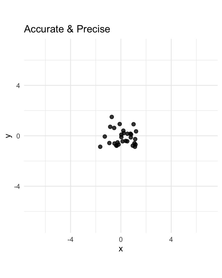
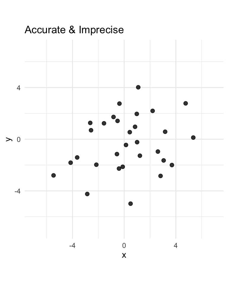
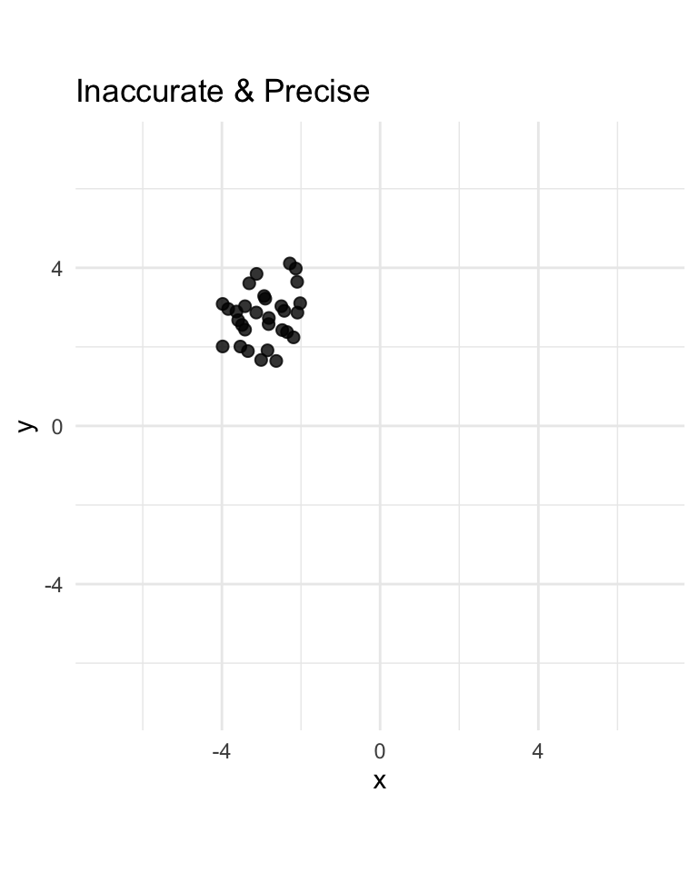
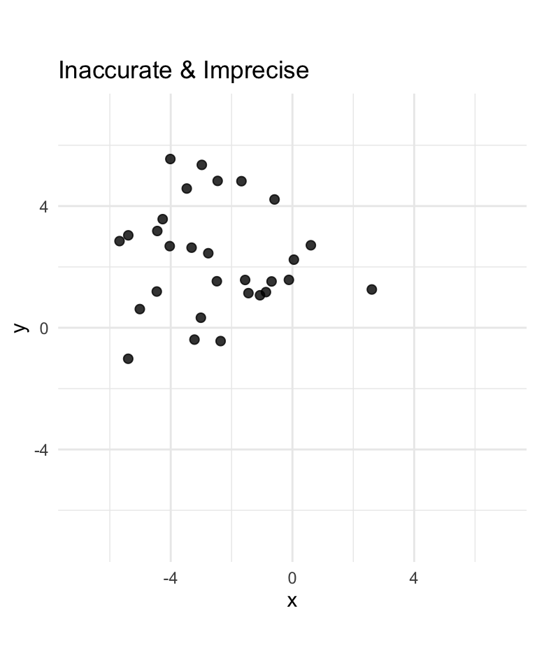
Therefore, we can clearly see that $V$ is biased from $\eqref{eq:v-bias}$. However, the MSE is actually the same as shown in $\eqref{eq:u-mse}$ and $\eqref{eq:v-mse}$. Therefore it is relatively hard to say which one is better. We see that $U$ is:

more accurate than $V$ (non-bias vs bias)
less precise than $V$ (since $c^2 / 6 > c^2 / 18$)
overall about as good as $V$ (since $c^2 / 6 = c^2 / 6$)

Since $U$ is unbiased and $V$ is not, we choose $U$ as the better of the two estimators. Does this mean that the estimate $V$ is useless? No. We can make use of $v$ as a starting point (or basis) for constructing an estimate that is better than $U$. Observe that $\E{V} = 2c/3$. This implies $\E{3V/2} = c$. So we define $W = 3V / 2.$ This is another estimator of $c$ to be considered. Now, what is the variance of $W$, \[\begin{equation*} \Var{W} = \left( \frac{3}{2} \right)^2 \Var{V} = \frac{9}{4} \cdot \frac{c^2}{18} = \frac{c^2}{8} \end{equation*}\] Therefore, we obtain the MSE as \[\begin{equation*} \mse{W} = \Var{W} = c^2/8 \end{equation*}\]

Now, we see that $W$ is:

just as accurate as $U$
more precise than $U$
overall better than $U$

We conclude that $W$ is best of the three estimators. So our best estimate of $c$ is $W = 1.5 \max(X,Y)$, our second best estimate is $U = X + Y$, and our third choice would be $V = \max(X, Y)$.

Something to be careful of…

Remark 1. Ideally, we should choose which estimator to use ($U$, $V$ or $W$) before observing the data ($X$ and $Y$).

4 Two Important Results for Estimation

Theorem 2 Suppose that $Y_1, Y_2, \ldots ,Y_n \sim^\iid (\mu, \sigma^2)$ and define $\mean{Y} = \frac{1}{n} \sum_{i=1}^n Y_i$ (sample mean) and $S^2 = \frac{1}{n-1} \sum_{i=1}^n (Y_i - \mean{Y})^2$ (sample variance). Then

$\E{\mean{Y}} = \mu$ (population mean)
$\E{S^2} = \sigma^2$ (population variance)

Proof (a). \[\begin{equation*} \E{\mean{Y}} = \frac{1}{n} \sum_{i=1}^n \E{Y_i} = \frac{1}{n} \sum_i^n \mu = \mu \end{equation*}\]

Proof (b). First, realise the following, \[\begin{equation*} S^2 = \frac{1}{n-1} \sum_{i=1}^n D_i^2 \hspace{10pt} \text{where $D_i = Y - Y_i$} \end{equation*}\]

Then, we can first find the second raw moment of $D_i^2$,

\[\begin{align*} \E{D_i^2} & = \Var{D_i} \tag{since $\E{D_i} = 0$} \\ & = \Var{Y_i} + \Var{\mean{Y}} - 2\Cov{Y_i, \mean{Y}} \\ & = \sigma^2 + \frac{\sigma^2}{n} - 2 \cdot \frac{\sigma^2}{n} \tag{Note 1} \\ & = \frac{n-1}{n} \sigma^2 \\ \end{align*}\]

Hence, \[\begin{equation*} \E{S^2} = \frac{1}{n-1} \sum_{i=1}^n \E{D_i^2} = \frac{1}{n-1} (n \cdot \frac{n-1}{n}\sigma^2) = \sigma^2 \end{equation*}\]

Note 1:

Note that we have previously shown $\mean{Y} \perp (Y_i - \mean{Y})$ for $\iid$ $Y_i$’s in Chpater 7 Section 2. Now, then, we have \[\begin{align*} 0 = \Cov{Y_i - \mean{Y}, \mean{Y}} & = \Cov{Y_i, \mean{Y}} - \Cov{\mean{Y}, \mean{Y}} \\ & = \Cov{Y_i, \mean{Y}} - \Var{\mean{Y}} \\ & = \Cov{Y_i, \mean{Y}} - \frac{\sigma^2}{n} \\ \end{align*}\]

Alternatively

In fact, we will see that $\iid$ is a relatively strong assumptions.

\[\begin{align*} \Cov{Y_i, \mean{Y}} &= \Cov{Y_1, \mean{Y}} = \Cov{ Y_1, \frac{1}{n}(Y_1 + Y_2 + \dots + Y_n) } \\ &= \frac{1}{n} \left( \Cov{Y_1, Y_1} + \Cov{Y_1, Y_2} + \dots + \Cov{Y_1, Y_n} \right) \\ &= \frac{1}{n} \left\{ \Var{Y_1} + 0 + 0 + \dots + 0 \right\} = \frac{\sigma^2}{n}. \\ \end{align*}\]

Hence, we know that $\Cov{Y_i, \mean{Y}} = \frac{\sigma^2}{n}$. In fact from the second proof, we also note that we don’t actually require

Corollary 1 (Unbias Estimator) Following directly from Theorem 2, we know that both $\mean{Y}$ and $S^2$ are unbias Estimator.

Theorem 3 (Sample Variance) \[\begin{equation*} S^2 = \frac{1}{n-1}\sum_{i=1}^n (y_i - \mean{y})^2 = \frac{1}{n-1}\left(\left(\sum_{i=1}^n y_i^2\right) - n\mean{y}^2 \right) \end{equation*}\]

Proof. The proof is almost identical to the proof for the analogous theorem of the population variance in Chapter 2 Section 2.1. Therefore, I will not restate here.