Sampling Distributions and Central Limit Theorem

1 Some Theorems Regarding the Normal Distribution

Theorem 1 Suppose that \(Y_1, Y_2, \ldots, Y_n \sim^{\text{iid}} N(\mu, \sigma^2)\). Let \[\bar{Y} = \frac{1}{n} \sum_{i = 1}^n y_i \hspace{20pt} \text{(the sample mean)}\]. Then \[\bar{Y} \sim N(\mu , \frac{\sigma^2}{n})\]

Proof. In Chapter 6, we showed that linear combinations of normal rv’s are also normal. So it only remains to find the mean and variance of \(\bar{Y}\).

\[ \begin{align} E[\bar{Y}] & = E\left[\frac{1}{n} \sum_{i = 1}^n Y_i\right] \\ & = \frac{1}{n} \sum_{i = 1}^n \mu = \frac{1}{n}n\mu = \mu Var(\bar{Y}) &= \frac{1}{n^2}\sum_{i=1}^n Var(Y_i) \\ &= \frac{1}{n^2} \sum_{i = 1}^n \sigma^2 \\ & = \frac{1}{n^2}n\sigma^2 = \frac{\sigma^2}{n} \\ \end{align} \]

2 Sampling Distribution

Corollary 1 (Standardised Sample Mean) \[ Z = \frac{\bar{Y} - \mu}{\sigma / \sqrt{n}} \sim N(0, 1) \]

\(Z\) may be called the standardised sample mean. The sample mean \(\bar{Y}\) is an example of a statistic

Definition 1 (Statistic) A statistic is any function of the observable random variables in a sample and known constants.

The probability distribution of a statistic is sometimes referred to as the sampling distribution of that statistic. For example, \(\bar{Y} - \mu\) is nto a statistic unless \(\mu\) is known. Similarly, \(Z\) in Corollary 1 is not a statistic unless both \(\mu\) and \(\sigma\) are known.

Example 1 A bottling machine discharges volumes of drink that are independent and normally distributed with standard deviation 1 ml.
Find the sampling distribution of the mean volume of 9 randomly selected bottles that are filled by the machine.
Hence find the probability that this sample mean will be within 0.3 ml of the mean volume of all bottles filled by the machine.

---

Let \(Y_i\) be the volume of the \(i\) th bottle in the sample, \(i = 1, \ldots, n\) where \(n = 9\). Then \(Y_1, Y_2, \ldots , Y_n \sim^{\text{iid}} N(\mu, \sigma^2)\), where \(\sigma^2 = 1\) and \(\mu\) is unknown. So \(\bar{Y} \sim N(\mu, 1/9)\). Hence

\[ \begin{align} P(\lvert \bar{Y} - \mu \rvert < 0.3) & = P(\left\lvert \frac{\bar{Y} - \mu}{\sigma / \sqrt{n}} \right\rvert < \frac{0.3}{1/3}) = P(\lvert Z \rvert < 0.9) \\ & = 1 - 2P(Z > 0.9) = 0.6318 \end{align} \]

It is important to note that we do not need any knowledge of \(\mu\). In fact, this is an example of a pivotal statistics.

---

Theorem 2 Suppose that \(Y_1, Y_2, \ldots , Y_n \sim^{\text{iid}} N(\mu, \sigma^2)\). Let \[ S^2 = \frac{1}{n-1}\sum_{i = 1}^n (Y_i - \bar{Y})^2 \] (The sample variance)

Then:

1. \[ \frac{(n - 1)S^2}{\sigma^2} \sim \chi^2(n-1) \]
2. \[ S^2 \perp \bar{Y} \]

---

Proof for (a)

Proof (a.). Although the proof is not assessable, but let’s give some intuitions why it works here. Note that this proof take idea from Mike Spivey answer to this question posted on StackExchange. Also, for this proof, let’s assume b. is true.

From Chapter 6, we know that the square of a normal distribution random variable will follow \(\chi^2\) distribution while sum of \(\chi^2\) distribution is still a \(\chi^2\) distribution but with higher degree of freedom.

With this intuition in mind, the only confusing point is why it is of \(n-1\) degree-of-freedom rather than \(n\). Now, we can first suppose that we know the parameters being \(\mathcal{N}(\mu, \sigma^2)\). Then, we can first consider \(\sum_{i=1}^n \left(\frac{Y_i - \mu}{\sigma}\right)^2\) \[ \begin{align} \sum_{i=1}^n \left( \frac{Y_i - \mu}{\sigma} \right)^2 & = \sum_{i=1}^n \left( \frac{(Y_i - \bar{Y}) + (\bar{Y} - \mu)}{\sigma} \right)^2 \\ & = \sum_{i=1}^n \left( \frac{Y_i - \bar{Y}}{\sigma} \right)^2 + \sum_{i=1}^n \left( \frac{\bar{Y} - \mu}{\sigma} \right)^2 + \sum_{i=1}^n \frac{2(Y_i - \bar{Y})(\bar{Y} - \mu)}{\sigma^2} \\ & = \frac{n-1}{\sigma^2} \left( \frac{1}{n-1} \sum_{i=1}^n (Y_i - \bar{Y})^2 \right) + n\left( \frac{\bar{Y} - \mu}{\sigma} \right)^2 + \frac{2(\bar{Y} - \mu)}{\sigma^2} \sum_{i=1}^n (Y_i - \bar{Y}) \\ & = \frac{n-1}{\sigma^2}S^2 + n \left( \frac{\bar{Y} - \mu}{\sigma} \right)^2 + \frac{2(\bar{Y} - \mu)(n\bar{Y} - n\bar{Y})}{\sigma^2} \\ & = \frac{n-1}{\sigma^2}S^2 + \left( \frac{\bar{Y} - \mu}{\sigma / \sqrt{n}} \right)^2 \\ \end{align} \]

Now, since we assumed b. is true, so \(\frac{n-1}{\sigma^2}S^2\) and \(\left( \frac{\bar{Y} - \mu}{\sigma / \sqrt{n}} \right)^2\) would be independent. Therefore, if we denote the above as \(V = U + W\) so \(U\) and \(W\) are indpendent, then \[ m_V(t) = m_U(t)m_W(t) \]

Now, then since the \[\frac{\bar{Y} - \mu}{\sigma /\sqrt{n}} \sim \mathcal{N}(0, 1) \implies \left( \frac{\bar{Y} - \mu}{\sigma / \sqrt{n}} \right)^2 \sim \chi^2(1) \implies W \sim \chi^2(1)\]. Also, since \[ \begin{align} Y_i \sim^{\text{iid}} \mathcal{N}(\mu, \sigma^2) & \implies \left( \frac{Y_i - \mu}{\sigma} \right) \sim^{\text{iid}} \mathcal{N}(0, 1) \\ & \implies \left(\frac{Y_i - \mu}{\sigma} \right)^2 \sim^{\text{iid}} \chi^2(1) \\ & \implies \sum_{i=1}^n \left(\frac{Y_i - \mu}{\sigma} \right)^2 \sim \chi^2(n) \\ & \implies V \sim \chi^2(n) \\ \end{align} \] Hence, arriving at the mgf of \(U\) being, \[ \begin{align} m_U(t) & = \frac{m_V(t)}{m_W(t)} \\ & = \frac{(1 - 2t)^{-n/2}}{(1 - 2t)^{-1/2}} \\ & = (1 - 2t)^{(-n / 2) + (1/2)} \\ & = (1 - 2t)^{-(n - 1) / 2} \\ \end{align} \] Hence, we see that this moment generating function is the same as \(\chi^2(n - 1)\). Hence, we know that \(U \sim \chi^2(n-1)\).

---

In order to prove (b), we need to first prove the following,

Lemma 1 (Independence of Centered Random Variables) Suppose \(Y_1, Y_2, \ldots , Y_n\) is a random sample iid from a normal distribution with mean, \(\mu\) and variance, \(\sigma^2\). It follows that the sample mean \(\bar{Y}\), is independent of \(Y_i - \overline{Y}\), \(i = 1, 2, \ldots, n\).

A Relatively Hard Proof for Lemma 1¹

Let’s first give some intuitions how to even start…

The idea of the following proof is essentially but using the fact that if the pdf of joint distribution of \(X_1, \ldots, X_N\) can be written as, \[f(x_1, x_2, \ldots, x_n) \propto g(x_1) h(x_2, \ldots x_n)\], then we can say that \(X_1\) is independent of \(\{ X_2, X_3, \ldots ,X_n\}\). Clearly, in this case \(X_1\) would be the sample mean, but how do we choose the others?

Proof (Lemma 1). The joint distribution of \(Y_1, Y_2, \ldots, Y_n\) is \[f_Y(y_1, y_2, \ldots, y_n) = \frac{1}{(2\pi)^{\frac{n}{2}}\sigma^n} exp \left\{ -\frac{1}{2} \sum_{i = 1}^n \left( \frac{y_i - \mu}{\sigma} \right)^2 \right\}\] Transform the random variables, \(Y_i, i = 1,2, \ldots , n\) to \[ \begin{align*} X_1 &= \overline{Y} & \quad \overline{Y} &= X_1 \\ X_2 &= Y_2 - \overline{Y} & \quad Y_2 &= X_2 + X_1 \\ X_3 &= Y_3 - \overline{Y} & \quad Y_3 &= X_3 + X_1 \\ \vdots &\;= \vdots & \quad \vdots &= \vdots \\ X_n &= Y_n - \overline{Y} & \quad Y_n &= X_n + X_1 \end{align*} \]

Then, the pdf is found through using the Jacobian of the transformation. In this context, the Jacobian (mapping from \(X\) to \(Y\) as we want to find the joint distribution of \(X\) and segregated it as suggested above) is, \[ [J_{ij}] = \left[\frac{\partial (Y_1, Y_2, \ldots Y_n)}{\partial (X_1, X_2, \ldots, X_n)}\right] = \begin{bmatrix} \frac{\partial Y_1}{\partial X_1} & \frac{\partial Y_1}{\partial X_2} & \cdots & \frac{\partial Y_1}{\partial X_n} \\ \frac{\partial Y_2}{\partial X_1} & \frac{\partial Y_2}{\partial X_2} & \cdots & \frac{\partial Y_2}{\partial X_n} \\ \vdots & \vdots & \ddots & \vdots \\ \frac{\partial Y_n}{\partial X_1} & \frac{\partial Y_n}{\partial X_2} & \cdots & \frac{\partial Y_n}{\partial X_n} \\ \end{bmatrix} = \begin{bmatrix} 1 & -1 & -1 & \cdots & 1 \\ 1 & 1 & 0 & \cdots & 0 \\ 1 & 0 & 1 & \cdots & 0 \\ \vdots & \vdots & \vdots & \ddots & \vdots \\ 1 & 0 & 0 & \cdots & 0 \\ \end{bmatrix} \]

Now, it only remains to find the determinant of \(J\). First, use row operations to achieve the following form, \[ J \sim \begin{bmatrix} 1 & -1 & -1 & \cdots & -1 \\ 0 & 2 & 1 & \cdots & 1 \\ 0 & 1 & 2 & \cdots & 1 \\ \vdots & \vdots & \vdots & \ddots & \vdots \\ 0 & 1 & 1 & \cdots & 2 \\ \end{bmatrix} \]

Therefore, we only need find the determinant of the bottom right \((n-1) \times (n-1)\) sub-matrix, \[ \lvert B\rvert \triangleq \left\lvert \begin{bmatrix} 2 & 1 & \cdots & 1 \\ 1 & 2 & \cdots & 1 \\ \vdots & \vdots & \ddots & \vdots \\ 1 & 1 & \cdots & 2 \\ \end{bmatrix} \right\rvert \]

Now, the easiest way is to realise the following, \[ B = 2I_{n-1} + (\mathbf{1}\mathbf{1}^\top - I_{n-q}) = I_{n-1} + \mathbf{1}\mathbf{1}^\top \] as a special case of the householder matrix.

Then, we realise the following eigendecompositions,

1. \(\mathbf{1} = \begin{bmatrix} 1 & 1 & \cdots & 1 \end{bmatrix}^\top\) is an eigen-vector of \(\mathbf{1}\mathbf{1}^\top\) with eigen-value \(n-1\).
2. Other orthogonal vectors to \(\mathbf{1}\) would also be eigenvectors, but with eigenvalues of 0. We generally have \(n - 1\) linearly independent such vectors. One example set is by considering using \(\{ \mathbf{e}_j - \mathbf{e}_1 \}\).

Therefore, \(B\) has eigenvalues, \[ \lambda_1 = 1 + (n - 1) = n, \qquad \lambda_2 = \cdots = \lambda_{n-1} = 1 \]

Hence, \[ \det B = n \cdot 1^{n-2} = n \]

Therefore, \(\lvert J \rvert = n\). Now, with a bit of detour, we know the pdf of joint distribution of \(Y_1, Y_2, \ldots , Y_n\) is \[ \begin{align} f_{X_1, X_2, \ldots , X_n}(x_1, x_2, \ldots , x_n) &= f_Y(y_1, y_2, \ldots, y_n) \lvert J \rvert \\ & = n f_X(y_1, x_1 + x_2, \ldots, x_1 + x_n) \\ & = \text{constants} \cdot \exp \left\{ -\frac{1}{2} \sum_{i=1}^n \left( \frac{y_i - \mu}{\sigma} \right)^2 \right\} \end{align} \] Now, something similar comes up again as above… \[ \begin{align} \sum_{i=1}^n \left( \frac{y_i - \mu}{\sigma} \right)^2 & = \frac{1}{\sigma^2} \sum_{i=1}^n (y_i - \mu)^2 \\ & = \frac{1}{\sigma^2} \left[ (y_1 - \overline{y})^2 + \sum_{i=2}^n (y_i - \overline{y})^2 + n(\overline{y} - \mu)^2 \right] \end{align} \] Note that since \(\sum_{i = 1}^n(y_i - \overline{y})\), it follows that \[ y_1 - \overline{y} = - \sum_{i=2}^n (y_i - \overline{y}) \]

Therefore, the above simpliifies to

\[ \begin{align} \sum_{i=1}^n \left( \frac{y_i - \mu}{\sigma} \right)^2 & = \frac{1}{\sigma^2} \left[ \left( \sum_{i=1}^n (y_i - \overline{y}) \right) ^2 + \sum_{i = 2}^n (y_i - \overline{y})^2 + n(\overline{y} - \mu)^2 \right] \\ & = \frac{1}{\sigma^2} \left[ \left( \sum_{i = 2}^n x_i \right)^2 + \sum_{i=2}^n x_i^2 + n(x_1 - \mu)^2 \right] \\ \end{align} \]

Therefore, the pdf of \(X_1, X_2, \ldots, X_n\), simplifies to \[ \begin{align} f_{X_1, X_2, \ldots, X_n}(x_1, x_2, \ldots , x_n) & = \text{constants} \cdot \exp \left\{ -\frac{1}{2\sigma^2} \left[ \left( \sum_{i=2}^n x_i \right)^2 + \sum_{i=2}^n x_i^2 + n(x_1 - \mu)^2 \right] \right\} \\ & \propto \exp \left\{ \frac{1}{2\sigma^2} \left[ \left( \sum_{i=1}^n x_i \right)^2 + \sum_{i=2}^n x_i^2 \right] \right\} \exp \left\{ -\frac{n}{2\sigma^2} (x_1 - \mu)^2 \right\} \\ & \propto h(x_2, x_3, \ldots , x_n) \cdot g(x_1) \\ \end{align} \]

Now, this follows with \(X_1\) being independent of \(X_2, \ldots, X_n\) as their joint probability distribution can be factored into a product of functions that depend only their repsectie set of statistics. Therefore, \(X_1 = \overline{Y}\) is independent of \(X_i = Y_i - \overline{Y}\), \(i = 2, 3, \ldots, n\).

Finally, since \(Y_1 - \overline{Y} = -\sum_{i=2}^n (Y_i - \overline{Y})^2\), it follows that \(Y_1 - \overline{Y}\) is a function of random variables that are independent of \(X_1 = \overline{Y}\), and so indpendent to \(X_1\).

Proof (b.). Now, all the hardwork is actually done in the proof of Lemma 1. The remaining parts requires to prove b. is essentially recognising that \(S^2\) is a function \(Y_i - \overline{Y}\) for \(i = 1, 2, \ldots , n\). Therefore, \(\overline{X}\) and \(S^2\) is independent.

Example 2 Similar setting as Example 1. Find an interval which we can be 90% sure will contain the sample variance of the 9 sampled volumes.

---

We will solve \(P(a < S^2 < b) = 0.9\) for \(a\) and \(b\).

\[ 0.9 = P\left(\frac{(9-1)a}{1} < \frac{(n-1)S^2}{\sigma^2} < \frac{(9-1)b}{1}\right) = P(8a < U < 8b) \] where \(U \sim \chi^2(8)\).

Then, using the \(\chi^2\) table, we obtain, \[ 0.9 = P(2.73264 < U < 15.5073) \] Therefore, we know that \(a = 0.34158\) and \(b = 1.9384125\). Hence, the required interval is \((0.34158, 1.93841)\).

Remark 1 (Is the above really the only solution?). Well, not really, it is relatively easy to find another interval. For example, we can find the interval starting from \(0\). In fact, a related problem is: “Find the shortest interval which we can be 90% sure will contain the sample variance of the 9 sampled volumes.”

The solution to this problem is unique and required interval \((a, b)\) satisfies two equations: \(P(a < S^2 < b) = 0.9\) and \(f_{S^2}(a) = f_{S^2}(b)\). This solution will have to be found numerically, e.g. trial and error or the Newton Raphson algorithm. This seemingly difficult problem is caused by the asymmetric of the probability density function.

2.1 The \(T\) Distribution

Definition 2 (\(t\) Distribution) Suppose that \(Z \sim \mathcal{N}(0, 1)\), \(Y \sim \chi^2(k)\) and \(Z \perp U\). We say that the random variable \[ Y = \frac{Z}{\sqrt{U/k}} \] where \(k\) being the only parameters has the \(t\)-distribution with \(k\) degrees of freedom. The pdf of \(Y\) is \[ f(y) = \frac{\Gamma(\frac{k+1}{2})}{\sqrt{k\pi}\Gamma(k/2)}(1 + \frac{y^2}{k})^{-\frac{1}{2}(k+1)} \hspace{10pt} , \hspace{10pt} \infty < y \infty \]

We write \(Y \sim t(k)\) or \(Y \sim t_k\)

Theorem 3 (Pdf of \(t\) Distribution) \[ f(y) = \frac{\Gamma(\frac{k+1}{2})}{\sqrt{k\pi}\Gamma(k/2)}\left(1 + \frac{y^2}{k}\right)^{-\frac{1}{2}(k+1)} \hspace{10pt} , \hspace{10pt} \infty < y \infty \]

The \(t\) pdf looks like a standard normal pdf but with ‘fatter’ tails. The \(t\) distribution converges to the standard normal distribution as \(k\) tends to infinity.

Theorem 4 (Convergence of the \(t\) Distribution) \(t\) distribution converges to standard normal distributions as degree of freedom tends to infinity.

Proof (Convergence to Standard Normal). The pdf of \(Y\) can be written \(f(y) = c_k A_k(y) B_k(y)\), where \(c_k\) is a constant (which does not depend on y), \[ A_k(y) = \left[ \left(1 + \frac{y^2}{k} \right)^k \right]^{-\frac{1}{2}} \qquad B_k(y) = \left( 1 + \frac{y^2}{k} \right) ^{-1/2} \] Now, as \(k \to \infty\), \(B_k(y) \to 1\) and \(A_k(y) \to \left[ e^{y^2} \right]^{-1/2} = e^{-\frac{1}{2} y^2}\). Therefore, as \(k \to \infty\), the pdf of \(Y \sim t(k)\) converges porportionally to \(e^{-\frac{1}{2}y^2}\), which is the kernel of the \(\mathcal{N}(0, 1)\).

In fact it is also possible to show that \(c_k \to 1 / \sqrt{2\pi}\). However, I think since we know that the results will be a probability density function, the only plausible \(c_k\) really can only be \(1 / \sqrt{2\pi}\).

Theorem 5 (Standardise with Sample Statistic) Suppose that \(Y_1, Y_2. \ldots , Y_n \sim^{\text{iid}} \mathcal{N}(\mu, \sigma^2)\). Let \[ T = \frac{\overline{Y} - \mu}{S / \sqrt{n}} \] Then, \(T \sim t(n-1)\).

Proof. Observe the following facts:

1. The standardised random variable with known variance by Corollary 1 is, \[Z = \frac{\overline{Y} - \mu}{\sigma / \sqrt{n}}\]
2. The sampling distribution of the sample variance by Theorem 2 is \[U = \frac{(n-1)S^2}{\sigma^2} \sim \chi^2(n-1)\]
3. \(Z \perp U\) by Theorem 2

It follows by definition of the \(t\) distribution that \[ Y = \frac{Z}{\sqrt{U/(n-1)}} \sim t(n - 1) \] But \[ T = \frac{\overline{Y} - \mu}{S / \sqrt{n}} = \frac{\frac{\overline{Y} - \mu}{\sigma / \sqrt{n}}}{\sqrt{\frac{(n - 1)S^2}{\sigma^2} / (n - 1)}} = Y \sim t(n-1) \]

---

Example 3 (T-statistic in action) Setting as Example 1. Find the probability that the mean of the \(9\) sample volumes will be distant from the population mean by no more than half the sample standard deviation of those \(9\) volumes.

\[ \begin{align} P\left(\left\lvert \overline{Y} - \mu \right\rvert < \frac{1}{2} S\right) & = P\left(-\frac{1}{2} S < \overline{Y} - \mu < \frac{1}{2} S \right) \\ & = P\left(-\frac{1}{2} < \frac{\overline{Y} - \mu}{S} < \frac{1}{2} \right) \\ & = P\left(-\frac{3}{2} < \frac{\overline{Y} - \mu}{S / \sqrt{n}} < \frac{3}{2} \right) \\ & = P\left( -\frac{3}{2} < T < \frac{3}{2} \right) \\ & = 1 - P(T < -1.5) \end{align} \]

Now, by tables, \(P(T < -1.397) = 0.1\) and \(P(T < -1.860) = 0.05\). Therefore, \(P(T < -1.5)\) is between \(0.05\) and \(0.10\). So \(1 - 2P(T < -1.5)\) is between \(0.8\) and \(0.9\).

2.2 The \(F\) Distribution

Definition 3 Suppose that \(U \sim \chi^2(a)\), \(V \sim \chi^2(b)\) and \(U \perp V\). We say that the random variable \(Y = \frac{U / a}{V / b}\) ahs the \(F\)-distribution with \(a\) numerator and \(b\) denominator degrees of freedom.

We write \(Y \sim F(a, b)\) or \(Y \sim F_{a, b}\).

Theorem 6 The pdf of an \(F\) distribution is \[ f(y) = \frac{\Gamma(\frac{a+b}{2})}{\Gamma(a/2)\Gamma(b/2)} a^{\frac{a}{2}}b^{\frac{b}{2}} y^{\frac{a}{2} - 1} (b + ay) ^{-\frac{1}{2}(a + b)} \; , \hspace{20pt} y > 0 \]

---

Theorem 7 \[ Y \sim F(a, b) \implies 1/Y \sim F(b, a) \]

Proof. Easily proved.

---

Theorem 8 (Sampling Distribution of Ratio of Sample Variance) Suppose that: \[ \begin{align} X_1, X_2, \ldots, X_n &\sim^{\text{iid}} \mathcal{N}(\mu_X, \sigma_X^2) \\ Y_1, Y_2, \ldots, Y_n &\sim^{\text{iid}} \mathcal{N}(\mu_Y, \sigma_Y^2) \\ (X_1, X_2, \ldots, X_n) &\perp (Y_1, Y_2, \ldots , Y_m) \\ \end{align} \]

Then \[ W = \frac{S_X^2 / \sigma_X^2}{S_Y^2 / \sigma_{Y}^2} \sim F(n-1, ,m-1) \] where \[ \begin{align} \overline{X} & = \frac{1}{n}\sum_{i=1}^n X_i \\ \overline{Y} & = \frac{1}{m}\sum_{i=1}^m Y_i \\ S_X^2 & = \frac{1}{n-1}\sum_{i=1}^n(X_i - \overline{X})^2 \\ S_Y^2 & = \frac{1}{m-1}\sum_{i=1}^m(Y_i - \overline{Y})^2 \\ \end{align} \]

Proof. By Theorem 2, \[ \begin{align} \frac{(n-1)S_X^2}{\sigma_X^2} & \sim \chi^2(n-1) \\ \frac{(m-1)S_Y^2}{\sigma_Y^2} & \sim \chi^2(m-1) \\ \end{align} \]

Both are indepndent of each other because the two samples are independent. Hence, by definition, \[ W = \frac{\frac{(n-1)S_X^2}{\sigma_X^2}}{\frac{(m-1)S_Y^2}{\sigma_Y^2}} \sim F(n-1, m-1) \]

---

Example 4 Same setting as Example 1. Suppose that another sample of \(5\) bottles is to be taken from the outpu of the same bottling machine. Find the probability that the sample variance of the volumes in these \(5\) bottles will be at least \(7\) times as large as the sample variance of the volumes in the \(9\) bottles that were initially sampled.

\[ \begin{align} P(S_X^2 \geq Y S_Y^2) & = P\left( \frac{S_X^2}{S_Y^2} > 7 \right) \\ & = P\left( \frac{S_X^2 / \sigma_X^2}{S_Y^2 / \sigma_Y^2} > 7 \right) \\ & = P(U > 7) \\ & \approx P(U > 7.01) = 0.010 \end{align} \]

Note that we can simply introduce \(\sigma_X\) and \(\sigma_Y\) because the two samples are know to from the same distribution and should, therefore, have the same population variance.

3 The Central Limit Theorem (CLT)

Theorem 9 (Central Limit Theorem) Suppose that \(Y_i, Y_2, \ldots , Y_n \sim^{\text{iid}} (\mu, \sigma^2)\), where \(-\infty < \mu < \infty\) and \(\sigma\) positively bounded. Let \[ U_n = \frac{\overline{Y} - \mu}{\sigma / \sqrt{n}} \implies U_n \xrightarrow{\text{d}} \mathcal{N}(0, 1) as n \to \infty \]

Note that we do not need to assume any distribution in this case, making it suitable for any sample without any assumed prior.

---

Example 5 200 numbers are randomly (uniformly) chosen from 0 and 1. Find the probability that the average of these number is greater than 0.53.

---

Solution 1

Let \(Y_i\) be the \(i\) th number, \(i = 1, \ldots , n\), where \(n = 200\). Then \(Y_1, Y_2, \ldots , Y_n \sim^{\text{iid}} U(0, 1)\). Thus \(\mu = 1/2\) and \(\sigma^2 = 1/12\). Since we know the population expectation, we can directly apply the CLT and find that, \[ P(\overline{Y} > 0.53) = P\left(\frac{\overline{Y} - \mu}{\sigma / \sqrt{n}} > \frac{0.53 - 0.5}{\sqrt{1/12} \sqrt{200}}\right) \approx P(Z > 1.47) = 0.0708 \] using normal tables.

How good is the normal approximation?

source("../../scripts/plot_bates.R")
print(bates_plot)

 

Warning: Using `size` aesthetic for lines was deprecated in ggplot2 3.4.0.
ℹ Please use `linewidth` instead.

 

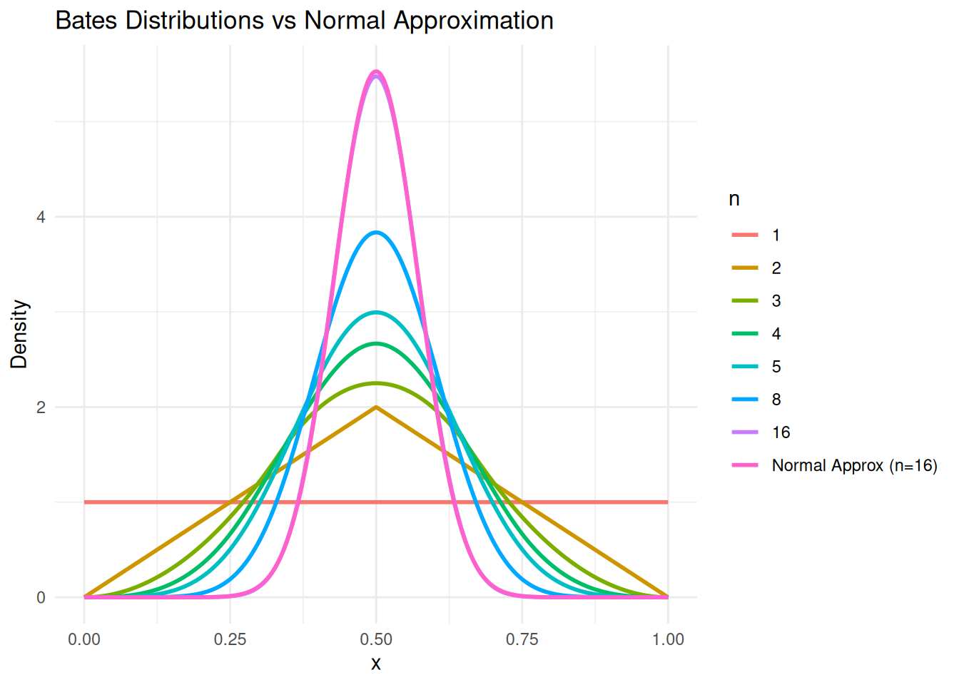
We can clearly see that this in fact as \(n\) becomes larger, it would become a better and better approximations. This is in fact called the Bates distribution, found by using convolution operator. Essetially, one can show that \[ f_{X_1 + X_2}(z) = \int_0^1 f_{X_1}(x)f_{X_2}(z - x) \, \mathrm{dx} \]

3.1 Alternative

Yet another way to think about the CLT is \(\sumrv{Y} \approx \NormalDist(n\mu, n\sigma^2)\), where \(\sumrv{Y} = Y_1 + Y_2 + \ldots + Y_n\)

Example 6 A dies is about to be rolled 50 times, and each time you will win as many dollars as the number which comes up. Find the probability that you will win a total of at least $200.

---

Solution

let \(Y_i\) be the number of dollars you will win on the \(i\)-th roll. Then \(Y_1, Y_2, \ldots, Y_n \; \iid (\mu, \sigma^2)\), where: \[\begin{align} \mu & = \E{Y_i} = 3.5 \\ \sigma^2 & = \Var{Y_i} = 2.9167 \\ \end{align}\]

Therefore, \(\P{\sumrv{Y} \geq 200} \approx \P{U > 200}\), where \(U \sim \NormalDist(50 (3.5), 50(2.9167)) = \NormalDist(175, 145.83)\).

Then \(\P{\dot{Y} \geq 200} \approx \P{Z > \frac{200 - 175}{\sqrt{145.83}}} = \P{Z > 2.07) = 0.0192\)

3.2 Normal Approximation to \(\Binomial(n, p)\)

Suppose that \(Y \sim \Binomial(n, p)\), then \(Y = Y_1 + Y_2 + \ldots + Y_n\), where \(Y_1, \ldots Y_2 \sim^\iid \Bernoulli(p)\). So \(Y_1, Y_2, \ldots, Y_n \; \iid (\mu, \sigma^2)\), where: \[\begin{gather*} \mu = \E{Y_i} = p \\ \sigma^2 = \Var{Y_i} = p(1 - p) \\ \end{gather*}\] It follows by the CLT that \(Y \approx \NormalDist(np, np(1 - p))\).

---

Example 7 (Normal Approximation (to everything?)) A die is rolled \(n = 120\) times. Find the probability that at least 27 sixes come up.

---

Solution

Let \(Y\) be the number of \(6\)’s. Then \(U \triangleq Y \sim \Binomial(120, 1/6)\). So \(Y \approx \NormalDist(120 (1/6), 120 (1/6)(5/6)\)

Hence, \[\begin{align*} \P{Z \geq 27} & \approx \P{U > 27} \\ & = \P{Z > \frac{27 - 20}{\sqrt{16.67}}} = \P{Z > 1.71} = 0.0436 \\ \end{align*}\]

3.2.1 The Continuity Correction

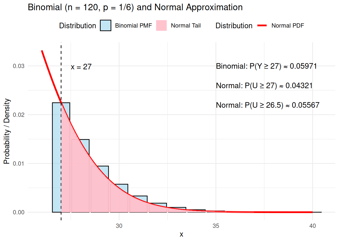
However, we need to take a closer look at the approximation made when we are applying to discrete cases. In Figure 1 below, the shaded red area is the area calculated as \(\P{U > 27}\) after normal approximation while the blue boxes underlay is the actual binomial distribution probability. Therefore, we can see that almost half of the column for \(x = 27\) is missed when we directly use the \(\NormalDist\). Hence, a better approximation would then be \[\begin{equation*} P(Y \geq 27) = P(U > 26.5) \end{equation*}\]

library(ggplot2)

# 參數設定
n <- 120
p <- 1/6
mu <- n * p
sigma <- sqrt(n * p * (1 - p))

# x 值
x_binom <- 27:40
x_norm <- seq(26, 40, length.out = 400)

# 分布
binom_probs <- dbinom(x_binom, size = n, prob = p)
norm_density <- dnorm(x_norm, mean = mu, sd = sigma)

# 資料框：每個都加上 'type' 欄位
df_binom <- data.frame(x = x_binom, y = binom_probs, type = "Binomial PMF")
df_norm <- data.frame(x = x_norm, y = norm_density, type = "Normal PDF")
df_shade <- data.frame(x = x_norm[x_norm >= 27],
                       y = norm_density[x_norm >= 27],
                       type = "Normal Tail")

# 1. Exact Binomial tail probability: P(Y ≥ 27)
p_binom <- sum(dbinom(27:n, size = n, prob = p))

# 2. Normal approximation without continuity correction: P(U ≥ 27)
p_norm_naive <- pnorm(27, mean = mu, sd = sigma, lower.tail = FALSE)

# 3. Normal approximation with continuity correction: P(U ≥ 26.5)
p_norm_corrected <- pnorm(26.5, mean = mu, sd = sigma, lower.tail = FALSE)

# Print results
# cat(sprintf("Binomial: P(Y ≥ 27) ≈ %.5f\n", p_binom))
# cat(sprintf("Normal Approx (naive): P(U ≥ 27) ≈ %.5f\n", p_norm_naive))
# cat(sprintf("Normal Approx (corrected): P(U ≥ 26.5) ≈ %.5f\n", p_norm_corrected))

# 畫圖
ggplot() +
  geom_col(data = df_binom, aes(x = x, y = y, fill = type), color = "black", width = 0.9, alpha=0.5) +
  geom_line(data = df_norm, aes(x = x, y = y, color = type), linewidth = 1.2) +
  geom_vline(xintercept = 27, linetype = "dashed", color = "black") +
  geom_area(data = df_shade, aes(x = x, y = y, fill = type), alpha = 0.95) +
  annotate("text", x = 27.5, y = max(df_norm$y)*0.9, label = "x = 27", hjust = 0, size = 4) +
  annotate("text", x = 35, y = 0.03,
           label = sprintf("Binomial: P(Y ≥ 27) ≈ %.5f", p_binom),
           hjust = 0, size = 4) +
  annotate("text", x = 35, y = 0.026,
           label = sprintf("Normal: P(U ≥ 27) ≈ %.5f", p_norm_naive),
           hjust = 0, size = 4) +
  annotate("text", x = 35, y = 0.022,
           label = sprintf("Normal: P(U ≥ 26.5) ≈ %.5f", p_norm_corrected),
           hjust = 0, size = 4) + 
  scale_fill_manual(
    name = "Distribution",
    values = c(
      "Binomial PMF" = "skyblue",
      "Normal Tail" = "pink"
    )
  ) +
  scale_color_manual(
    name = "Distribution",
    values = c(
      "Normal PDF" = "red"
    )
  ) +
  labs(
    title = "Binomial (n = 120, p = 1/6) and Normal Approximation",
    x = "x", y = "Probability / Density"
  ) +
  theme_minimal() +
  theme(legend.position = "top")

Figure 1: Why we need to have continuity correction?

# Parameters
n <- 120
p <- 1/6
mu <- n * p
sigma <- sqrt(n * p * (1 - p))

Footnotes

1. This proof is in reference to this material published by the Duke University which I found on Google somehow. If this material should not be public, please contact me with details here